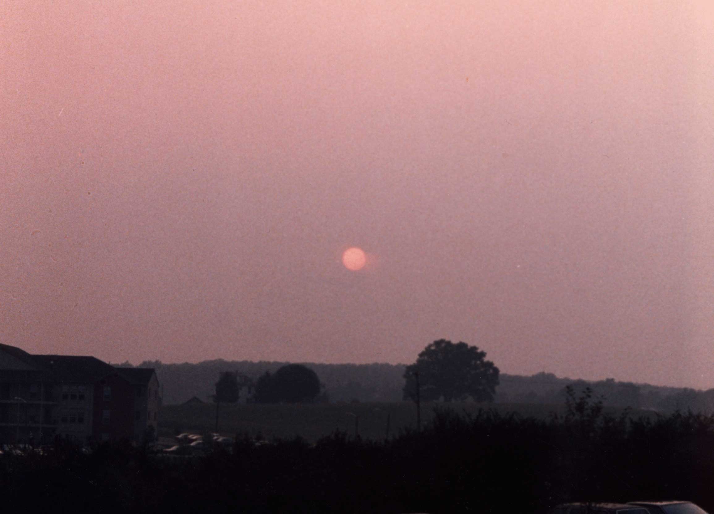
Figure 1. The setting sun dimmed by dense haze over
State College, Pennsylvania on 16 September 1992.
Haze Over the Central and Eastern United States
(Originally published in the National Weather Digest, Mar. 1996;
Updated Dec. 2004, Feb. 2009, Jan. 2012, Sep. 2012, and Jun. 2013;
Photographs by the author)
Abstract
The origin and nature of warm season haze over the central and eastern United
States are discussed. Summarizing the results of various studies dating to
the mid-1970s, the microphysical basis of haze is described, with emphasis on
the fact that a large component of haze appears to be anthropogenic. The synoptic
meteorology of haze is then presented. It is shown that over the central and eastern
United States, haze most often is associated with modified polar air, not
tropical air, as commonly is believed. Forecasting the movement of haze areas using
850 mb trajectories is demonstrated by example. The paper concludes with a
discussion of haze-free "tropical surge" events along the East Coast.
Outline of paper
1. Introduction
2. The nature of haze
a. Haze as pollution
b. Haze chemistry
(1) SO2 and sulfates
(2) Formation of sulfate aerosols
(3) Growth of sulfate aerosols and their appearance as haze
(4) The natural component
3. Haze climatology
a. A summer phenomenon
b. Why the East is hazy
c. Haze in the West
4. Forecasting haze
a. Introduction
b. A typical example
c. Early season haze
d. Haze and tropical cyclones
5. Tropical surges
6. Concluding remarks
7. Footnotes
8. Acknowledgements
9. References
1. Introduction
During summer, the central and eastern United States often is blanketed by a
murky veil of haze that may last for days. The haze shrouds the sky and dims the
sun --- sometimes making it altogether disappear before the end of the day
(Figure 1). To some, haze is so commonplace that it is assumed to be natural and
is accepted as a fact of life.
But haze is, in fact, not predominantly natural, and its presence warrants attention
for several reasons. For example, haze affects human health. Researchers at New York
University Medical Center have determined that the acid droplets found in haze
are hazardous to exposed tissues of the lungs and breathing passages (Pendick
1993). They also concluded that when haze occurs in association with smog ---
the brownish, photochemically-enhanced form of air pollution derived from automobile
exhausts --- the destructive nature of that phenomenon significantly is increased.
Haze also affects aviation. While not posing an overwhelming risk to jet aircraft,
haze shrouds visual cues important to pilots of small planes. When widespread, haze may
significantly reduce visual range over thousands of square miles. Haze, in fact,
likely was a factor in the fatal crash of the small plane piloted by John F. Kennedy, Jr.,
near Martha's Vineyard, Massachusetts in July 1999.
Figure 1. The setting sun dimmed by dense haze over
State College, Pennsylvania on 16 September 1992.
Haze, however, does more than limit visibility and impair health. The same airborne compounds resposible for haze also produce acid rain (Urone and Schroeder 1978, Husar 1990). As a result, haze is linked to the acid precipitation-induced demise of Douglas fir trees in the eastern United States (Mitchell 1994), as well as to the accelerated crumbling of concrete, mortar, and statuary.
Numerous studies have shown that clouds that form in hazy air, on average, produce less rainfall than those that evolve in less contaminated environments (Monastersky 1992). In addition, when present in patches or bands, haze can affect the strength and distribution of surface heating. In this manner, haze can subsequently influence patterns of convective development and regional precipitation (e..g, Lyons 1980).
Evidence also is mounting that haze plays a significant role in determining the global energy balance, since it not only diminishes the amount of solar energy reaching the surface, but also reduces the rate at which the atmosphere radiates longwave energy to space (Ball and Robinson 1982, Penner et al. 1994). One study concluded that because of haze, some parts of the eastern United States experience an annual solar radiation deficit of about 7.5% (Ball and Robinson 1982). A more recent estimate by William Chameides of the Georgia Institute of Technology (Raloff 1999) suggests that the reduction of photosysnthesis due to haze in China could be robbing that country of more grain than the entire nation imports.
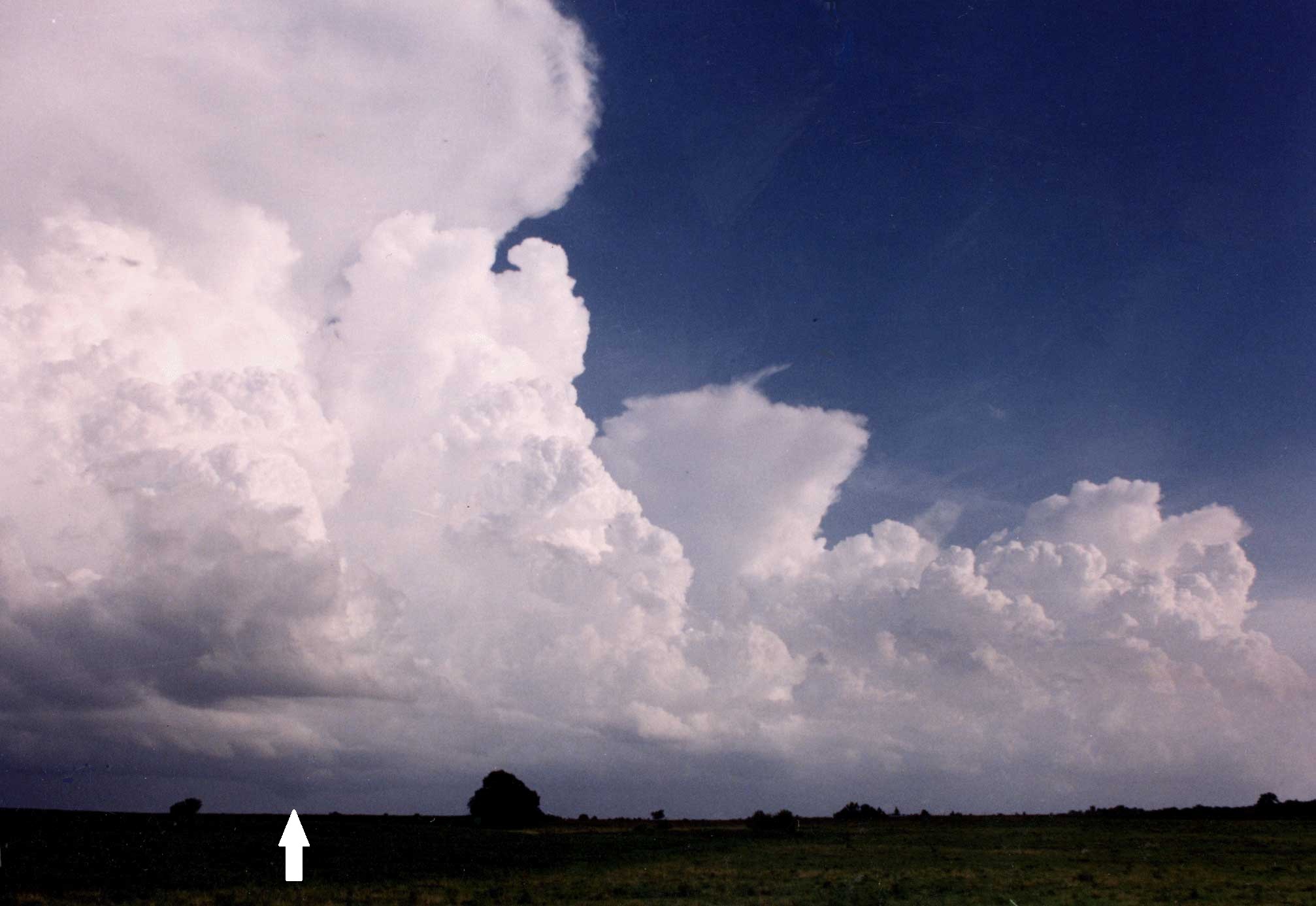
Another reason that haze is of interest is aesthetic: Haze affects the clarity with
which we view the environment (e.g., Hyslop 2009). Haze can obscure not only the
daytime sky (Figure 2), but also the stars, the Milky Way, and other features of the
nighttime heavens. Rainbows, haloes, and vivid sunset colors all fade when haze shrouds
the view. Haze also robs the landscape of contrast and hue. A tree-studded scene that
seems to glow with color on a clear fall afternoon in New England loses its luster on
a day with haze. And, while haze does add depth to distant vistas and mountain scenery,
ordinary scattering by air molecules and dust will do the same without the loss
of color and visual range associated with haze.
 |
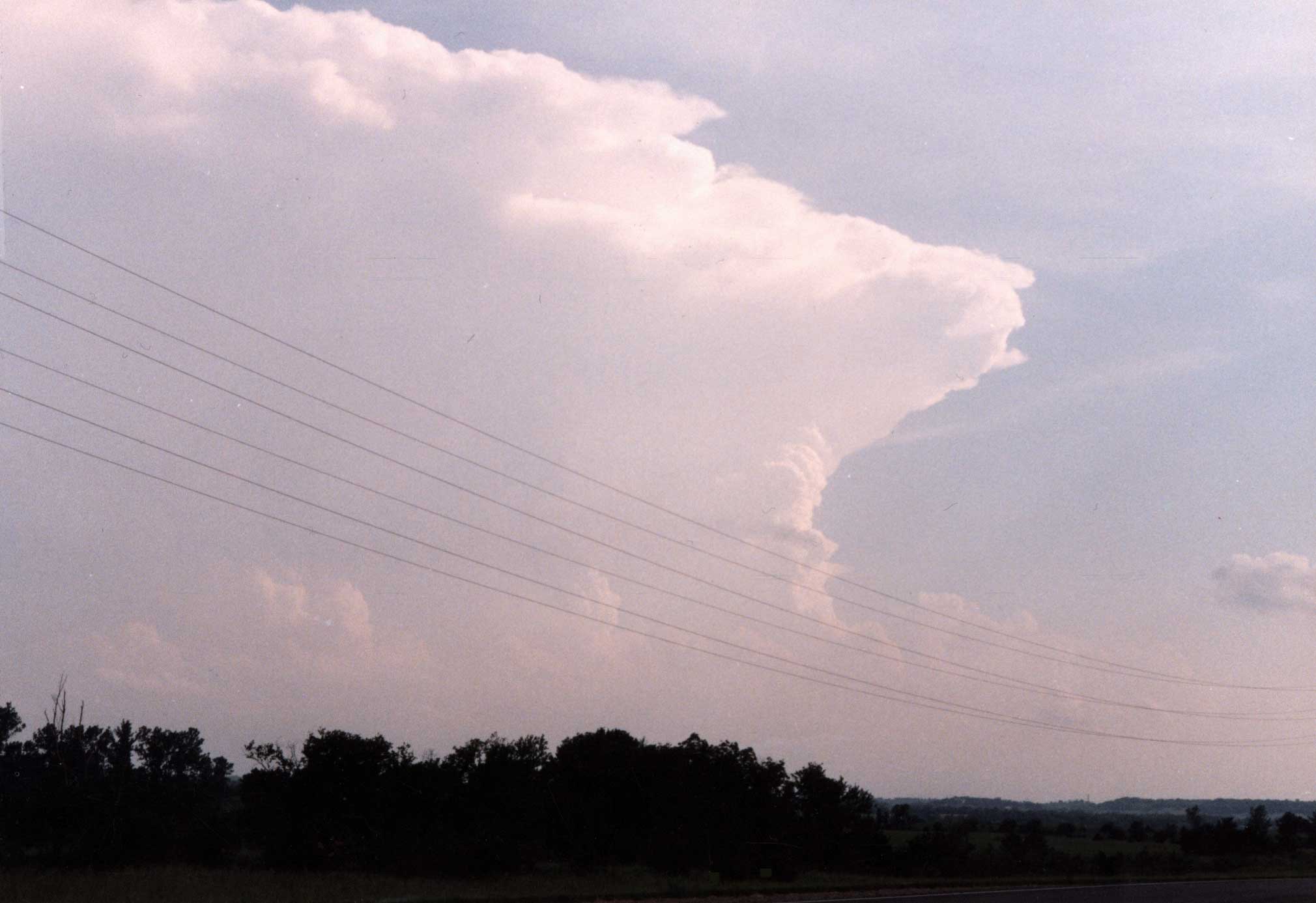 |
Figure 2. Haze can hinder severe weather spotting, as demonstrated by this pair of photographs of supercell thunderstorms viewed from similar distances (approximately 25 miles), similar directions (south-southeast), and at similar times (early evening). In the left image, the main updraft base is visible, including a wall cloud (mesocyclonic lowering) above the arrow at the lower left (12 July 1986 near Sedalia, Missouri). In the right view, the main updraft base is obscured by haze (7 June 1990 near Topeka, Kansas). Tornadoes occurred shortly after both photographs were made.
The reduction in visual quality caused by haze, however, is more than cosmetic. Campbell (1983), Evans and Cohen (1987), and Zeidner and Shechter (1988) all indicate that poor visual air quality causes heightened levels of anxiety, tension and depression in humans. In a similar study, Jones and Bogat (1978) linked increased interpersonal aggression and hostility to reductions in visual air quality.
In summary, the impact of haze, though sometimes subtle, is quite significant. Yet for many, and, to a surprising extent, even within the meteorological community, haze remains a poorly understood phenomenon. This paper addresses development and movement of haze over the central and eastern United States, with emphasis on its largely anthropogenic origin. Much of the material has been presented elsewhere, but for the most part in sources not widely available to operational meteorologists.
2. The nature of haze
a. Haze as pollution
As previously noted, haze often is assumed to be natural, with evapotranspirative
products from trees being the most oft-cited source. Others attribute haze to the
minute particles of salt released during the breaking of ocean waves. Popular
meteorological works (e.g., Ludlum 1991) perpetuate this view, using the term "haze"
to refer strictly to natural obstructions to vision.
Certainly natural forms of haze do exist. But, as the following pages show,
the type of haze commonly seen over the eastern half of the United States during
summer is not predominantly natural. Haze is, in fact, primarily a vast blanket of
man-made pollution. More specifically, haze is a form of "wet" air pollution ---
a veil of tiny droplets (aerosols) of condensed pollutants.1 The
adjective "wet" is used to distinguish this type of haze from the dry forms
that consist of fine dust particles and more commonly are observed elsewhere in
the world (e.g., the "Harmattan" of west Africa, or the shamal wind haze of
the Persian Gulf).
Numerous studies since the mid-1970s (see, for example, Ferman et al. 1981,
Wolff et al. 1982, Malm 1992, Husar and Wilson 1993, Chen et al. 2003) consistently
have shown that warm-season haze over the eastern United States is composed largely
of sulfate aerosols. To understand the formation of sulfate aerosols, then, is
to understand the formation of warm-season haze.
b. Haze chemistry
(1) SO2 and sulfates
Sulfates are sulfur-based compounds that contain sulfate ions (ions of the
form SO42-). The sulfates that comprise haze aerosols are
derived mainly from the oxidation of sulfur dioxide (SO2) and may
exist in solid or liquid form. Airborne sulfates also originate from bursting
air bubbles in ocean waves and, over arid regions, from the abrasion of
sulfate-bearing soils by the wind (Wallace and Hobbs 1977). But these two sources
produce comparatively large particles (over 2.0 um in diameter) that, like salt
particles from ocean waves, settle rapidly and do not represent a major
source of haze aerosols.
Since haze-producing sulfates originate from SO2, a few words are
in order regarding the origin and nature of atmospheric SO2. Sulfur
dioxide is a colorless gas that has the odor of burning sulfur. It may be both
natural or anthropogenic (man-made). Most natural SO2 is produced from
the oxidation of hydrogen sulfide gas (H2S), a by-product of vegetative
decay. Volcanoes are another significant natural source of SO2 (de Pena 1982).
Anthropogenic SO2 is produced in great quantity during the
large-scale combustion of sulfur-bearing fossil fuels in power plants, oil
refineries, and steel mills. Lesser amounts are produced during the manufacture
of pulp and paper. In United States, SO2 emissions are concentrated
along the "industrial crescent" extending from the mid-Mississippi Valley east
into the lower Great Lakes and mid-Atlantic states (Figure 3). A separate
SO2 source region is associated with oil production along the upper
Texas and Louisiana Gulf Coasts.
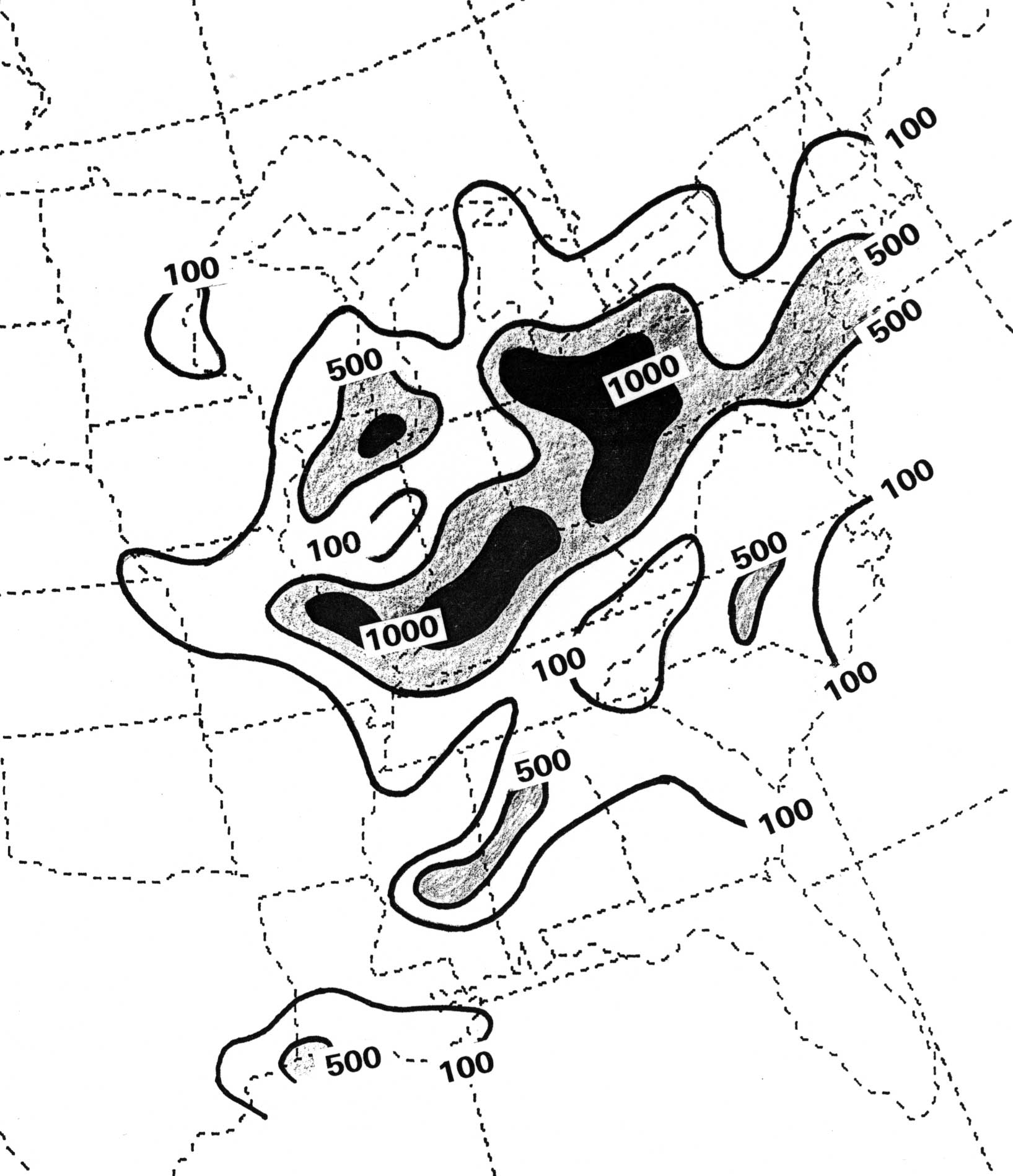
Figure 3. Distribution of SO2 emissions during summer over the eastern United States in metric tons per day (After Brueske 1990).
Nearly 2.7 x 10⁷ metric tons of SO2 are produced in the United States each year, about one fourth of the world's total output (Brueske 1990). Coal-burning power plants in the Ohio Valley alone yearly contribute 3 million tons (Malm 1992). Worldwide, man-made SO2 emissions increased nearly 30-fold between the mid-1800s and the mid-1900s as a result of industrial development (Heicklen 1976).
Even in highly polluted environments, the concentration of SO2 in
the atmosphere rarely exceeds 1 part per million; over rural areas average
concentrations are on the order of one part per billion. More than half,
however, of the SO2 over continental areas is thought to be
anthropogenic, compared to about one third for the atmosphere as a whole (de
Pena 1982). This is especially true over the northern hemisphere, where more
than 90% of the total man-made output is produced (Heicklen 1976). A more
precise estimate of the total anthropogenic component of SO2 over a
given area is difficult to ascertain because of lingering unknowns in the many
sulfur budget equations involved.
(2) Formation of sulfate aerosols
The oxidation of SO2 in the atmosphere can occur in
different ways. Some of these paths include only gas-phase reactions, while
others involve exclusively liquid-phase reactions or some combination of the
two. Those paths that result in the formation of sulfate aerosols are known as
"gas-to-particle conversions," since they involve the formation of liquid or
solid aerosols from a gas.
For example, one gas-phase SO2 oxidation path involves oxidation
of SO2 to form gaseous sulfuric acid (H2SO4).
The latter gas is then converted to a liquid sulfate aerosol either by contact with
existing aerosols or by serving as a nuclei for the condensation of water vapor
(Rogers and Yau 1989). In contrast, liquid-phase oxidation of SO2 occurs
inside cloud droplets after the gas has become dissolved in them.
Because gas-to particle conversions typically require the presence of
secondary pollutants such as ozone (O3), conversion reactions are
usually enhanced by sunlight. Reaction rates also vary with relative humidity.
For example, the oxidation rate of SO2 to sulfate increases by a
factor of eight when the relative humidity increases from 70 to 80% (Wallace and
Hobbs 1977).
The particular type of sulfate that forms during the oxidation of
SO2 is dependent on not only whether the reaction occurs in the gaseous
or liquid phase, but also on the degree of neutralization that occurs during
the oxidation process. Neutralization, in turn, is governed by the number and
type of cations (positive ions) present during the reaction. Ammonium, calcium,
sodium and magnesium are the most common neutralization ions. For example,
complete neutralization by ammonium produces ammonium sulfate
((NH4)2SO4), whereas partial neutralization results in the
formation of ammonium bisulfate ((NH4)HSO4). The
production of sulfuric acid (H2SO4), meanwhile, represents
a complete absence of neutralization.
Even with some neutralization, the sulfates found over the eastern United
States tend to be very acidic. These particles generally exist as aqueous nitric
and sulfuric acid, the result of gas-phase reactions during which gaseous acids
are converted to liquid forms by the addition of water vapor. It is the
downstream transport of these aerosols, and their eventual elimination from the
atmosphere in the form of acid rain and snow, that results in the low pH
(hydrogen ion concentration) characteristic of precipitation over the
Appalachians and much of the remainder of the East.2
(3) Growth of sulfate aerosols and their appearance as
haze
All sulfate aerosols, depending upon their degree of neutralization, are at
least somewhat hygroscopic. This means that they adsorb water molecules from the
environment, even when the relative humidity is below 100 percent. As a result,
sulfates are excellent condensation nuclei. The aerosols grow (deliquesce) as
water vapor condenses on them, and they continue to grow until they reach a size
at which they are in equilibrium with their environment.3
If the environment is supersaturated with respect to water, sulfate droplets
eventually reach such a size that they become readily visible as a cloud. If,
however, the humidity in their vicinity is somewhat lower, say around 85
percent, the droplets might grow to only about .5 um in diameter. This is about
one tenth the size of most cloud droplets but may be twice the diameter of the
aerosol before it was "wetted." Aerosols of this size are in the range (.1 um to
1 um) over which scattering efficiency per unit particle mass reaches a maximum
(National Research Council 1990); in fact, particles of this size scatter
visible sunlight a million times more effectively than air molecules. Figure 4
illustrates graphically the relationship between scattering by aqueous sulfate
aerosols and increasing relative humidity.

Figure 4. Effect of relative humidity on the scattering of visible light by liquid sulfate aerosols, as measured by extinction coefficient, bext. Extinction coefficient is a measure of the attenuation of a beam of light as a result of scattering or absorption in a medium. (After Ferman et al. 1981).
The scattering of sunlight by molecules in the atmosphere is a form of Rayleigh scattering. Rayleigh scattering is a general term for the scattering produced by particles that are very small compared to the wavelength of the incident light. The degree of scattering that occurs is inversely proportional to the fourth power of the wavelength involved. Thus, because blue light is of a shorter wavelength than red (.39 vs. .76 um), a sky dominated by Rayleigh scattering by air molecules appears blue.4
In contrast to the scattering of sunlight by air molecules, the scattering
produced by hygroscopic sulfate aerosols is not wavelength-dependent. Because
such particles are comparable in size to the wavelength of light, the scattering
they produce is a complex function of particle size and wavelength. If the
aerosols are all the same size, the sky might take on a faint red or blue hue
depending on the size of the aerosols and on whether the part of the sky being
viewed is seen by scattered or transmitted light. But if a range of aerosol
sizes exists, as is most often the case, no particular color is favored and the
sky appears white (reflecting a loss of spectral purity in the scattered light).
In addition, because the aerosols represent a net increase in the total number of
particles that naturally would be present in the atmosphere, the tendency for
whitening is further increased. These extra particles also enhance the atmospheric
absorption (attenuation) of sunlight --- and therefore reduce the amount of light
that reaches the ground. This effect is most notable at sunrise or sunset and is
responsible for the early fading of the sun noted in Figure 1.
(4) The natural component
Because haze is such a familiar sight in the eastern U.S. and has no obvious
source, casual observers find it difficult to believe that it is not natural in
origin. Some will note that the Blue Ridge and Smoky Mountains were named long
before the widespread industrial use of fossil fuels. Indeed, a small percentage
of the particles found in haze are derived from volatile hydrocarbons such as
terpenes that are released by certain trees (Chang 1990). In addition,
atmospheric sulfates are not entirely anthropogenic.
But studies dating to at least 1940 show an incontrovertible link
between industrial sulfur emissions and the degree of haziness over the eastern
U.S., as shown, for example, in Figure 5 (Husar 1990, Malm 1992).5
And, research conducted in the Blue Ridge mountains has shown that
naturally-occurring aerosols are responsible for no more than 20% of the total
light extinction due to haze (Ferman et al. 1981). The primary reason for this
is that most organic aerosols (such as those from trees) are relatively
hydrophobic and therefore do not grow to such a size that they become visible as
haze.

Figure 5. Comparison of long-term sulfur emissions and degree of summertime haziness (as measured by extinction coefficient) over the southeastern United States. (From Malm 1992).
The Ferman study estimated that if all natural sources of pollution in the East were taken together, surface visibility would still exceed 25 miles --- well above the 4 to 6 mile visual range characteristic of summer afternoons over the region today. If any haze were visible at all, it would be of the thin, "blue" variety first noted by the Cherokee Indians in the early 1700s (Powell 1968) --- not the murky pall that frequently obscures the Blue Ridge mountains today. Accounting for the mean warm-season airflow over the East in summer, the study concluded that "observed airflow patterns are consistent with previous findings that Midwestern [sulfate] source areas are a major cause of widespread summertime haze in the eastern U.S."
More recent studies have continued to support these ideas, attributing more
than three quarters of summertime light extinction in the central Appalachians
to sulfates (Malm 1992, Sisler et al. 1993). This is not too surprising
considering Malm's observation that the average sulfate concentration over the
eastern states is some 5 to 10 times greater than the estimated natural
backround value of approximately .8 ug/m3 (Ferman 1981, Trijonis et
al. 1991). In addition, considering the hygroscopic nature of sulfate aerosols,
the finding by Chen at al. (2003) that water was responsible for about 40% of
the light extinction in a July 1999 sulfate haze event in the Baltimore-Washington
area also seems reasonable.
3. Haze climatology
a. A summer phenomenon
Sulfate aerosols are both small and chemically stable. As a result, they
settle only very slowly and can remain airborne for days. Most are eventually
washed from the atmosphere in the form of acid rain. Although sulfate
aerosols are formed wherever the precursor gas-to-particle conversion reactions
occur, it is synoptic- and regional-scale weather conditions that govern their
overall concentration and, thus, the occurence and persistence of haze.
Because large scale atmospheric transport reaches a minimum during summer,
insolation is at a maximum, and boundary layer humidity is enhanced by
evapotranspiration, sulfate haze primarily is a warm-season phenomenon. As
Figure 6 shows, haze in the United States is most common east of the Mississippi
River. Note that haze is less frequently observed over south Florida and northern
New England --- areas farther removed from major SO2 source regions and
areas more likely to experience air of a less contaminated origin. The data also
show an overall trend for increased haziness, especially over the
Southeast. This reflects the increased summertime use of bituminous coal for
electrical purposes such as air conditioning (Husar and Patterson 1980).
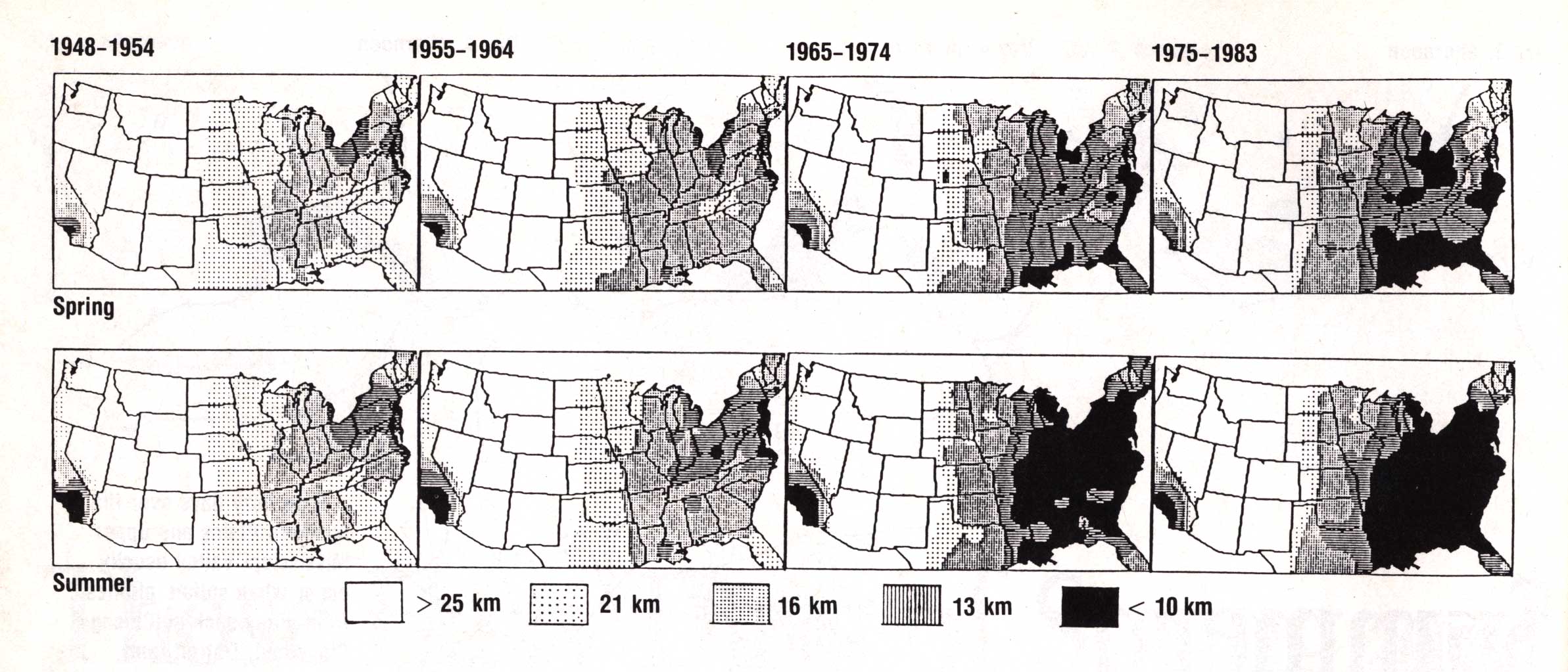
Figure 6. Long-term spatial distribution of haze (expressed as average visibility in km) over the United States. Top row: spring (April-June); bottom row, summer (July-September). (From Husar 1990).
b. Why the East is hazy
Proximity to the semi-permanent Bermuda anticyclone makes the eastern third
of the United States especially prone to prolonged episodes of synoptic-scale
sulfate haze in summer for reasons that already have been discussed. Large scale
transport over the central and eastern states reaches a minimum during July and August. Air
parcels originating over the lower Mississippi Valley, for example, may take three or four days
to reach the eastern Great Lakes or mid-Atlantic region. Vertical mixing also is often quite
limited, especially east of the Appalachians where subsidence is enhanced closer to
the mean position of the anticyclone. This increases the atmosphere's loading of both
SO2 and its sulfate oxidation products. In addition, because summer days are
long and large-scale cloudiness is at a minimum, evapotranspiration and photo-enhanced
gas-to-particle conversions can proceed at a maximum rate.
The source region of the air commonly present over the Midwest and East in
summer is another notable factor associated with the development of haze. While the Gulf
of Mexico often is blamed for the oppressive summertime combination of heat,
haze, and humidity ("The Three Hs") often present there, examination of surface air parcel
trajectories reveals that, in most cases, hazy air masses do not originate over
the Gulf, but rather are of continental polar origin. Such air masses most recently have
been resident over Texas, the lower Mississippi Valley, and the southeastern states, and have
undergone strong modification in their lowest layers. Because these air masses have had a
recent history of subsidence, an inversion often is present around 850 mb. The inversion
traps moisture added by evapotranspiration --- and haze aerosols generated locally --- in
the shallow boundary layer near the ground, while cleaner, drier conditions persist aloft.
The low "lid" placed on the top of the haze layer enhances its negative impact on visibility
and encourages additional aerosol growth as the air masses return poleward following summertime
cool air outbreaks. True Gulf (or tropical) air, in contrast, typically lacks a strong low-level
subsidence inversion and is characterized by modest thermodynamic instability through a comparatively
deep layer. As a result, any haze that may be present is mixed through that deeper layer and
made less dense.
The top of a haze layer in a modified polar air mass often is quite distinct. The
resulting "haze horizon" is a familiar sight to airline passengers over the central and eastern
states in summer. The "horizon," of course, marks the top of the polluted boundary layer. Because
relative humidity reaches a local maximum at the top of this well-mixed layer, haze is densest ---
and visual range is most reduced --- at an altitude just below that of the "horizon."
The reduction of visual range is most pronounced in the direction of the sun (where forward
scattering of sunlight is maximized), and is a well-known hazard of small-plane pilots.
6
c. Haze in the West
Much of the western United States is comparatively free of sulfate haze because
SO2 emissions are lower and the climate is dry. In addition, because the
air often is of recent oceanic origin, it tends to be "cleaner" (e.g., contains fewer
background particles) than the continental air typically present over the eastern
United States. As Figure 6 shows, however, haze does occur over some parts of the
West, and its occurrence gradually has increased in recent years (Malm 2000). In particular,
ozone smog and nitrate-based haze plague much of southern California in and around the Los
Angeles basin. These forms of pollution primarily are derived from motor vehicle emissions
(Sisler 1993), and have been traced to episodes of reduced visual range in the Grand Canyon and
other national parks of the southwestern states.
4. Forecasting haze
a. Introduction
The National Weather Service and WX-TALK (WeatherTalk) Web discussion group
postings from the 1990s shown in Figure 7 capture the frustration and
lack of understanding posed by haze from a forecasting perspective. Accurate
forecasting of haze remains problematic to this day. Although studies dating
to the mid-1970s have documented the growth and movement of sulfate haze
"blobs" over the eastern United States (see, for example, Hall et al. 1973,
Gillani and Husar 1976, Lyons et al. 1978, Husar et al. 1981, Wolff et al. 1981,
or Wolff et al. 1982), little of this material was written for or has found its
way into the operational environment. The following sections offer a
distillation of some of the more meteorologically-relevant material presented in
those papers. Information also is provided on the how different synoptic patterns
affect the development and movement of regional haze.

Figure 7. Selected forecast discussions mentioning haze from (a) the Birmingham, Alabama (0900 UTC 21 July 1991), and (b) Taunton (Boston), Massachusetts National Weather Service Forecast Offices (1930 UTC 21 July 1994 and 0140 UTC 22 July 1994); (c) excerpt of "WXTALK" blog on haze (14 August 1994). The Boston discussions reflect forecast thinking prior to and just after the passage of a typical "tropical surge" (See Section 5). Those parts of the discussions most relevant to haze appear in boldface.
From what already has been presented, it is apparent that haze forms wherever the sources of atmospheric sulfates overwhelm the sinks. This is why haze usually is associated with regions of large-scale stagnation. With both vertical and horizontal mixing at a minimum, whatever aerosols may be present will accumulate at first locally and then regionally over those areas experiencing minimal air flow, sunshine, and high relative humidity.
Favorable conditions for haze formation are realized on a regular basis each
summer over the SO2 source regions of the central and eastern United
States, two or three days after a polar air mass has settled over the area and
surface winds have become light. Under sunny skies, evapotranspiration can
result in substantial moistening of the boundary layer in the previously dry air
mass. Surface dewpoints that may have fallen into the 40s (degrees F) with cold
frontal passage may rebound to around 60 by the end of the second or third day.
Because conditions are favorable for rapid aerosol growth, and because the aerosols
are confined to a shallow boundary layer, haze may become noticeable as soon as 48
hours after a polar air mass has stagnated over the eastern United States.
b. A typical example Because eastern haze generally is confined to the lowest 7 or 8 thousand feet
above the surface, its movement over a period of days generally is well-correlated
with the streamlines of flow at 850 mb (Wolff et al. 1981). Figure 8 depicts the
progress of a typical summertime haze event over the east-central United States,
with the areas of haze shown as shaded areas on the 850 mb charts.
In this case, a mass of hazy air that formed in an old modified polar air mass over
the Ohio Valley was first shunted south to the Gulf Coast states ahead of a weakening
cold front (14-16 August). Once over the Gulf Coast, the air mass stalled and
picked up an additional load of sulfates from the refineries of southeast Texas and
Louisiana. The hazy air then made a return visit to the Ohio Valley as it was
drawn northward ahead of a new cold front over the central Plains and upper
Mississippi Valley (17-18 August). In such a manner, especially dense areas of haze
may form as sulfate aerosols accumulate in a given mass of air that makes one or more
return visits to an SO2 source region.
As is apparent in Figure 8, haze tends to concentrate in bands parallel to
fronts. This might seem perplexing considering that the depth of the boundary
layer tends to be greatest in the vicinity of fronts. But because large scale
ascent and low-level convergence are maximized there as well, relative humidity
also is at a maximum near fronts. Thus, sulfate production is enhanced and those
aerosols that do form grow to a comparatively large size. Weak fronts are
sometimes detectable in visible data satellite imagery when their associated
haze bands appear as a discontinuities in the brightness field.
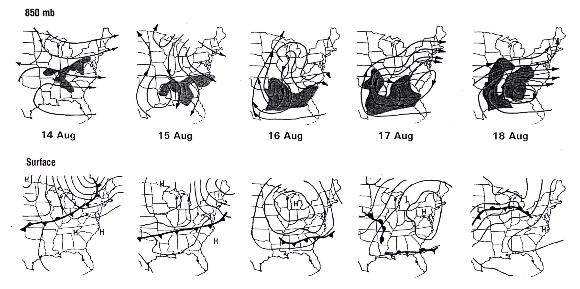
Figure 8. A haze "blob" that twice affects the lower Ohio Valley in August 1979. Haze areas (visual range less than 10 km) shaded, with 850 mb streamlines (top row) and surface isobars/fronts (bottom). Map times: 1200 UTC (After Wolff et al. 1981).
The case shown in Figure 8 also illustrates the importance of trajectory analysis to forecasting haze movement. Trajectory analysis is used to determine air parcel motion forward or backward in time from a specific point or region (Yarnal 1991). Because the formation of haze is not an instantaneous process, and because haze can be advected from one area to another, knowledge of an air mass' recent history is essential to making an accurate forecast of haze movement. For example, in this event, a forecaster in Peoria, Illinois, knowing that haze was reported earlier in the week at Little Rock and Memphis, should not be surprised by the appearance of haze over northern Illinois on 18 August. Even though the 850 mb flow over Illinois on the 18th was rather strong and from the west --- conditions not normally associated with haze in that part of the country --- back trajectories reveal that the air mass entering the state was indeed the same one that had brought haze to Arkansas and Tennessee two days earlier.
In contrast to the mid-Mississippi Valley, it is in fact not uncommon for brisk westerly winds to accompany haze over the eastern Great Lakes and New England. Notable haze episodes in the Northeast often occur in conjunction with mid-summer heatwaves and moderate to strong westerly flow on the northern fringe of an elongated Bermuda High. The enhanced westerly flow frequently is associated with the approach of a shortwave trough over the Saint Lawrence Valley. The winds, typically strongest ahead of a west-east cold front associated with the trough, tap dense haze areas that may have been developing under nearly perfect sulfate- forming conditions over the Ohio Valley for several days. When the "blobs" arrive in New York or New England, often it is just in time to produce a fall of acid rain as thunderstorms erupt along the front.
Once an area of haze has developed, it remains in existence until the aerosols are
washed out by rain. Dry deposition of haze (see Footnote 1) is minimal. Evidence also
suggests that boundary layer sulfates may be "vented" through the anvils of mesoscale
convective systems (McNaughton et al. 1994). Qualitative evidence certainly indicates
that surface visibilities increase in the wake of most mesoscale convective complexes and
larger mesoscale convective systems. In contrast, although isolated thunderstorms may rid
the boundary layer of local buildups of pollutants, visibility often is not improved
because the increase in boundary layer humidity in the vicinity of such storms enhances
the growth of remaining aerosols.
c. Early season haze
Observations show that surface dewpoints in the 60s most often are associated
with the onset of haze in the summer, since lower dewpoints at that time of year
are indicative of fresh outbreaks of polar air. But haze can occur with lower
dewpoints, especially during spring and fall. A classic example of "low dewpoint
haze" is illustrated in Figure 9. This event occurred in early April with
surface dewpoints in the 40s and temperatures in the 60s. The haze clearly was
not derived from natural sources such as trees since very little plant growth
was in progress at the time of the event due to unusually cold weather during
the preceding weeks.

Figure 9. Surface fronts and streamlines associated with an early season haze event (12-15 April 1992) over the north central states. Haze areas (as reported in surface airway observations) are shaded.
The main haze "blob" formed in a zone of persistent easterly flow north of a
west-east stationary front, where vertical mixing was limited by presence of a
strong frontal inversion (Figure 10). The sulfates likely originated in the
industrial area surrounding the lower Great Lakes and were carried west along
the southern fringe of a large polar anticyclone which had invaded the area earlier
in the week. Pollution from Chicago, Cleveland, Detroit, and Milwaukee contributed
to the haze that spread as far west as the Nebraska high plains.

Figure 10. SkewT-logP diagram for Topeka, Kansas, 0000 UTC 14 April 1992. Temperature and dewpoint lines solid and dashed, respectively; wind speeds in knots. Sounding shows pronounced frontal inversion near 875 mb.
As Figure 9 shows, the haze formed in modified polar air, not tropical air;
the haze-producing air mass never moved south of the Ohio River. It is also
worth noting that some of the haze that affected the north central states
during this event did, however, arrive from the south --- in the form of a
returning "blob" that had moved into Arkansas and Oklahoma with a cold
frontal passage earlier in the week.
d. Haze and tropical cyclones
Some of the most pronounced haze episodes in the central and eastern United States
are associated with the blocking of polluted air masses over the Ohio or
Mississippi Valleys when tropical cyclones are present along the East Coast.
Figure 11 shows how a mass of hazy air that formed over the Ohio Valley was forced
to remain over that region for two additional days as Hurricane "David" (1979) moved
north along the Eastern Seaboard (4-6 September). Once David reached New England,
northwest winds in the wake of the storm carried the heavy pollution load southward
behind a cold front into the Carolinas, Georgia, and the Gulf Coast states
(7-8 September). The GOES 7 satellite depiction of a more recent hurricane-related
haze event is shown in Figure 12. In this case ("Emily" 1993), northeast winds on the
fringe of the tropical system drove a plume of dense haze that had been resident over
the mid-Atlantic states southwest into the Carolinas.
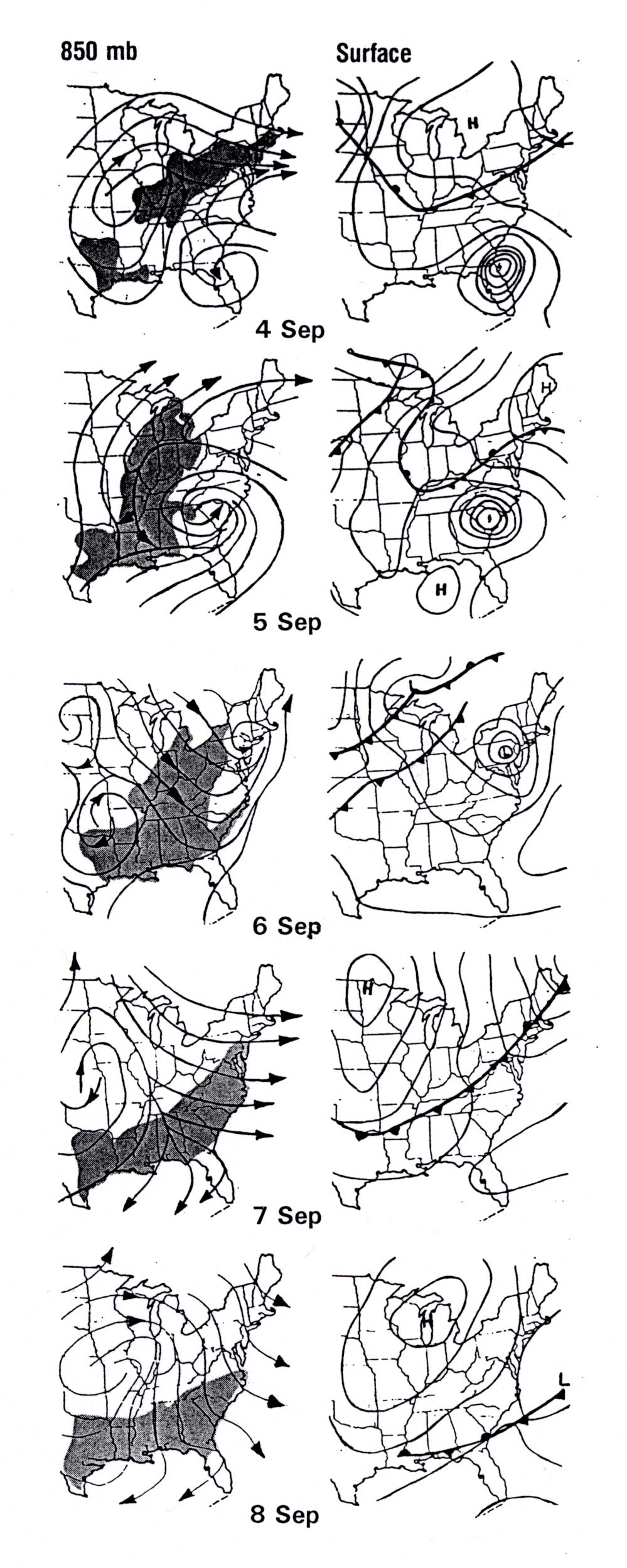
Figure 11. Surface (right column) and 850 mb (left column) evolution during a haze event influenced by Hurricane "David," September 1979. Map times: 1200 UTC; haze areas (visual range less than 10 km) depicted by shading. "David" is marked by circulation that moves northeastward from Florida to Pennsylvania. (After Wolff et al. 1982).

Figure 12. GOES 7 visible data view of the eastern United States at 1331 UTC 30 August 1993 showing Hurricane "Emily" over the western Atlantic and an extensive area of clear but hazy skies (light grey areas) covering much of the eastern United States. Over the central Appalachians and along the mid-Atlantic coast, a band of dense haze is being driven southwest into the Carolinas ahead of a "back-door" cold front on the northwest fringe of Hurricane "Emily."
Even in the absence of tropical cyclone activity it is not uncommon for haze
to follow the passage of weak cold fronts over the Gulf Coast states, the southern
Plains, and the Southeast. This is because the post-frontal air typically originates
over the Ohio Valley or lower Great Lakes. Embryonic sulfate aerosols born in these
SO2 source regions move south with the subsident post-frontal flow,
eventually growing into haze as they encounter increased sunshine and moisture
over the Gulf Coast and southeastern states.
5. Tropical surges
One of the more pleasant though uncommon characteristics of the normally hazy
summer months over the mid-Atlantic States and the Northeast is the arrival of
pure subtropical air from the western Atlantic in the form of a "tropical
surge." These events occur when the main axis of the Bermuda High rotates
decidedly clockwise from its usual west-east orientation along 30 or 35 degrees north
latitude. This may happen in response to the development of a strong trough over
the Mississippi Valley, or in response to the formation of a closed cyclonic circulation
along the south Atlantic Coast. Both scenarios result in deep and sustained south to
south-southwest flow over the mid-Atlantic States and the Northeast (Figure 13).

Figure 13. Standard NCEP 500 mb analyses associated with tropical surge events over the mid-Atlantic States. In the first case (top; 1200 UTC 4 August 1974), anomalous southerly flow along the eastern seaboard is related to an unusually deep trough over the Mississippi Valley. In the second (bottom; 1200 UTC 4 August 1988), a closed circulation east of Georgia produces a south to southeast flow along the mid- Atlantic Coast. Ridge axes are depicted by serrated lines.
Having had a long over-water trajectory, air streams of this type tap relatively
clean, sulfate-free source regions over the western Atlantic and Caribbean. Thus,
despite their high moisture content, they arrive in the northeastern United States
remarkably haze-free --- in marked contrast to the murky air masses they replace.
Because the maritime boundary layer usually is somewhat buoyant, cumulus buildups dot
the sky; some of these occasionally grow into thunderstorms. An example of a tropical
surge sky is given in Figure 14 (from Corfidi 1993). A stronger-than-normal
southerly component to the wind frequently accompanies surge events at the surface.

Figure 14. A "tropical surge" sky seen looking east from near Danville, Virginia around 1100 LST 14 July 1990. The azure blue sky and brightly-lit cumulus tops are characteristic of surge events. The boundary layer in this case is especially transparent (note that cloud details are apparent all the way to the horizon), even though surface dewpoints were in the 70s.
A series of surface observations depicting the midday arrival of a tropical
surge at Wilmington, Delaware on 20 July 1994 is shown in Figure 15. This
particular set of observations was chosen because it illustrates the
increase in visual range that occurs during a surge in the absence of a major
change in dewpoint. The sequence is also largely free of diurnal effects. In
this case, visibility increased from 5 miles in haze at noon local time (1550
UTC) to 12 miles at 6 pm (2150 UTC). The dewpoint, meanwhile, remained in the
mid-70s.
Figure 15. Sequence of surface airway observations depicting the arrival of a tropical surge at Wilmington, Delaware (station identifier ILG) around 1900 UTC (2 PM LST) 20 July 1994. Visibility (in statute miles, with "H" signifying observed haze) and dewpoint (in degrees F) given in the eighth and eleventh columns, respectively, from the left.
The doubling of visual range is significant since typically little or no visibility change is to be expected over this region on a summer afternoon in the absence of a frontal passage. In a sense, of course, a frontal passage did occur --- a mass of strongly modified continental polar air with a high sulfate content was replaced by cleaner air of Carribean or west Atlantic origin.
Surge "fronts," unfortunately, are not easily diagnosed by even the most sophisticated of today's objective analysis techniques. For example, the arrival of a surge generally produces no detectable change in surface equivalent potential temperature (theta-e). Automation of the surface observation network has exacerbated the detection problem since minimal information is now recorded regarding visibility changes above 6 miles. While the advance of a tropical surge sometimes can be tracked by satellite7, clouds often interfere with the view.
The 500 mb analysis sequence for the Wilmington surge event is shown in
Figure 16. In this case, the combination of a seasonably strong trough over the
upper Great Lakes with a weaker trough along the south Atlantic Coast together
produced anomalously deep southerly flow along the mid-Atlantic coast. Backing
of the upper flow as far north as Pennsylvania and New York on 21 July allowed
the surge to sweep northeast into New England the following day (Figure 16d).
Arrival of the surge in this area was rather abrupt, and elicited the comments
from the Boston area National Weather Service office shown in Figure 7b.
 |
 |
| a. | b. |
|
|
|
| c. | d. |
Figure 16. Standard NCEP 500 mb analyses for 1200 UTC (a) 19
July, (b) 20 July, (c) 21 July and (d) 22 July 1994 showing
evolution of mid-level flow during the tropical surge event depicted in Figure 15. The
surge reached Wilmington, Delaware on the 20th, and southern New England the
following day.
On average, tropical surges occur about once each summer along the mid-Atlantic Coast. They are, however, notably absent during some years (e.g. 1992 and 1993), while several events occur in others (e.g., 1994 and 2004). Their frequency necessarily decreases from south to north along the eastern seaboard, and their effects usually do not extend very far west of the central and northern Appalachians. Tropical surges also are observed in the deep South, when the large scale circulation allows Caribbean or western Atlantic air to overspread the Gulf Coast states (note comment regarding east-to-west flow in the forecast discussion shown in Figure 5a).
Surge events usually come to an end with the approach of a shortwave trough
in the westerlies. When these systems are weak, their passage is marked by only
a modest veering of the mean tropospheric flow. This shunts the maritime air
mass east into the Atlantic, allowing hazy, continental air from the lower Great
Lakes or Ohio Valley to return. If the shortwave is seasonably strong, however,
a more decided veering of the large scale flow will occur. This will usher in an
air mass of a more northerly origin, and the haze-free maritime flow will be
replaced by a relatively clean air mass from Canada.
6. Concluding remarks
The origin and nature of sulfate haze over the central and eastern United States have been presented. Misconceptions about the phenomenon have been examined, and information provided to better anticipate its formation and movement. Although the human impact of haze is not immediate like that posed by a tornado, flash flood, or hurricane, the long-term affects of haze are no less significant.
The incidence of sulfate haze has decreased over parts of the Midwest and Northeast in recent years due to the loss of industry and to a reduction in the use of high-sulfur coal in those areas (Husar 1990, Schichtel et al. 2001). And, in the Southeast, SO2 emissions have decreased as a result of stricter air pollution standards imposed by the 1970 Clean Air Act and its amendments.
But continued population growth and the increased demand for electrical power suggest
that haze will be with us for some time to come. In addition, regional haze that is not
predominantly sulfate-based but still traceable to anthropogenic sources has begun to affect
visibility in the national parks of Arizona and Utah (National Research Council 1990,
Sisler et al. 1993). Haze also is increasing in rapidly developing parts of the world such as
China, India, and southeast Asia (Che et al. 2007) --- and some of this haze reaches the United
States. Haze, therefore, will remain a challenge to the meteorological community --- a challenge
to not only better understand the phenomenon, but to also heighten awareness of its nature and
significance.
7. Footnotes
1. Technically speaking, the term "aerosol" refers to a system
consisting of particles suspended in a gas. Here, however, aerosol will be used
in its more popular sense to refer to the particles themselves.
2. Sulfate aerosols and gases may also exit the atmosphere via dry
deposition --- the deposit of airborne particles and gases on the earth
in the absence of precipitation.
3. Aerosol growth can also occur via coagulation, the process whereby
droplets that bump together adhere and subsequently merge into one droptlet (Malm
1992).
4. Theoretically, Rayleigh scattering should produce a violet sky since that
color has the shortest wavelength in the visible spectrum. But because human
eyes are most sensitive to the middle part of the spectrum, a clear sky appears
blue.
5. Similar regional trends have been observed elsewhere in the world (e.g.,
western Europe and China).
6. The "haze horizon" sometimes can be observed indirectly from the ground
as a dark band on the flanks of cumulus towers that penetrate beyond the
boundary layer. The dark band marks the angle of maximum light extinction due
to haze between the observer and the cloud.
7. In cloud-free areas, the remote detection of haze and other forms of
pollution improved significantly with the commissioning of next generation
satellites GOES 8 and GOES 9 (See Menzel and Purdom 1994). While not specifically
devoted to the tracking of haze or surge events, a site maintained by
the Atmospheric Lidar Group of the University of
Maryland - Baltimore County may be used to monitor haze and air pollution on a
national basis via satellite.
8. Acknowledgements
The author would like to thank Dr. Dennis Lamb (The Pennsylvania State University) and
three anonymous reviewers who substantially enhanced the clarity and technical content of
an early version of this paper. Thanks also to Steve Weiss (NOAA Storm Prediction Center)
for helpful comments, and to Karen Bennett, Sarah Corfidi, Roger Edwards, and Ryan Jewell
for HTML assistance.
9. References
Ball, R. J., and G. D. Robinson, 1982: The origin of haze in the central United States and its effect on solar radiation. J. Appl. Meteor., 21, 171-188.
Brueske, S. L., 1990: Forecasting atmospheric particulate sulfur concentrations using National Weather Service synoptic charts. Master's thesis, The Pennsylvania State University, 132 pp.
Campbell, F. W., 1983: Ambient stressors. Environ. Behavior, 15, 355-380.
Chang, J. S., 1990: Acid deposition: State of the science and technology. Report 4. National Acid Precipitation Assessment Program (especially pp 27-34).
Che, H., X. Zhang, Y. Li, Z. Zhou, and J.J. Qu, 2007: Horizontal visibility trends in China 1981-2005. Geophys. Res. Lett., 34, L24706, (doi:10.1029/2007GL031450).
Chen, L.-W. A., J. C. Chow, B. G. Doddridge, R. R. Dickerson, W. F. Ryan, and P. K. Mueller, 2003: Analysis of a summertime PM2.5 and haze episode in the mid-Atlantic region. Air & Waste Manage. Assoc., 53, 946-956.
Corfidi, S. F., 1993: Lost horizons. Weatherwise, 46, 12-17.
de Pena, R. 1982: Sulfur in the atmosphere and its role in acid rain. Earth and Mineral Sciences, 51, 62-66 (Available from College of Earth and Mineral Sciences, The Pennsylvania State University, University Park)
Evans, G. W., and S. V. Jacobs, 1981: Air pollution and human behavior. J.Social Issues, 37, 95-125.
Ferman, M. A., G. T. Wolff, and N. A. Kelly, 1981: The nature and sources of haze in the Shenandoah/Blue Ridge Mountains area. J. Air Pollut. Control Assoc., 31, 1074-1082.
Gillani, N. V., and R. B. Husar, 1976: Synoptic scale haziness over the eastern U.S. and its long range transport.
Proceedings of the 4th National Conference on Fire and Forest Meteorology, St. Louis, Missouri, 232-239.
Hall, F. P., C. E. Duchon, L. G. Lee, and R. R. Hagan, 1973: Long- range transport of air pollution: A case study, August 1970. Mon. Wea. Rev., 101, 404- 411.
Heicklen, J., 1976: Atmospheric Chemistry. Academic Press, 406 pp.
Husar, R. B., 1990: Historical visibility trends. Acid Deposition: State of Science and Technology. Report 24. National Acid Precipitation Assessment Program, 68-76.
-----, and D. E. Patterson, 1980: Regional scale air pollution: Sources and effects. Ann. NY Acad. Sci., 338, 399- 417.
-----, and W. E. Wilson, 1993: Haze and sulfur emission trends in the eastern United States. Environ. Sci. Tech., 27, 12-16.
-----, J. M. Halloway, D. E. Patterson , and W. E. Wilson, 1981: Spatial and temporal pattern of eastern U.S. haziness: A summary. Atmos. Environ., 15, 1919-1928.
Hyslop, N. P., 2009: Impaired visibility: The air pollution people see. Atmos. Environ., 43, 182-195.
Ludlum, D. M., 1991: The Audubon Field Guide to the Atmosphere. Alfred A. Knopf. 656 pp.
Lyons, W. A., 1980: Evidence of transport of hazy air masses from satellite imagery. Ann. NY Acad. Sci., 338, 418-433.
-----, J. C. Dooley Jr., and K. T. Whitby, 1978: Satellite detection of long-range pollution transport and sulfate aerosol hazes. Atmos. Environ., 12, 621-631.
Malm, W. C., 1992: Characteristics and origins of haze in the continental United States. Earth-Sci. Rev., 33, 1-36.
-----, 2000: Introduction to Visibility. Cooperative Institute for Research in the Atmosphere (CIRA), Colorado State University, 68 pp.
McNaughton, D.J., N. E. Bowne, R. L. Dennis, R. R. Draxler, S. R. Hanna, T. Palma, S. L. Marsh, W. T. Pennell, R. L. Peterson, J. V. Ramsdell, S. T. Rao, and R. J. Yamartino, 1994: Summary of the 8th Joint Conference on Applications of Air Pollution Meteorology. Bull. Amer. Meteor. Soc., 75, 2303-2311.
Menzel, W. P., and J. F. W. Purdom, 1994: Introducing GOES-I: The first of a new generation of geostationary operational environmental satellites. Bull. Amer. Meteor. Soc., 75, 757-781.
Mitchell, J. G., 1994: Legacy at risk. National Geographic, 186, 20-55 (October).
Monastersky, R., 1992: Haze clouds the greenhouse. Sci. News, 141, 232-233.
National Research Council, 1990: Haze in the Grand Canyon: An evaluation of the winter haze intensive tracer experiment. National Academy Press, 97 pp.
Pendick, D., 1993: Hazy summer days boost respiratory ailments. Sci. News, 143, pg 52.
Penner, J.E., R. J. Charlson, J. M. Hales, N. S. Laulainen, R. Lefier, T. Novakov, J. Ogren, L. F. Radke, S. E. Schwartz, and L. Travis, 1994: Quantifying and minimizing uncertainty of climate forcing by anthropogenic aerosols. Bull. Amer. Meteor. Soc., 75, 375-400.
Powell, W., 1968: North Carolina Gazeteer. University of North Carolina Press, Chapel Hill, North Carolina.
Raloff, J., 1999: Sooty air cuts China's crop yields. Sci. News, 156, pg 356.
Rogers, R. R., and M. K. Yau, 1989: A Short Course in Cloud Physics, 3rd ed. Pergamon Press. 290 pp.
Schichtel, B. A., and R. B. Husar, S. R. Falke, and W. E. Wilson, 2001: Haze trends over the United States, 1980-1995. Atmos. Environ., 35, 5205-5210.
Sisler, J. F., D. Huffman, and D. A. Latimer, 1993: Spatial and temporal patterns and the chemical composition of the haze in the United States: An analysis of data from the IMPROVE network, 1988-91. (Available from CIRA-Cooperative Institute for Research in the Atmosphere, Colorado State University, Ft. Collins, Colorado 80523)
Trijonis, J., R. Charlson, R. Husar, W. C. Malm, M. Pitchford, W. White, 1991: Visibility: Existing and Historical Conditions - Causes and Effects. In: Acid Deposition : State of Science and Technology. Report 24. National Acid Precipitation Assessment Program.
Urone, P. and W. H. Schroeder, 1978: "Atmospheric chemistry of sulfur-containing pollutants," Chapter 6 in Sulfur in the Environment, Part 1, J. O. Nriagu, ed. New York: Wiley Interscience.
Wallace, J. M. and P. V. Hobbs, 1977: Atmospheric Science: An Introductory Survey. Academic Press, 467 pp.
Wolff, G. T., N. A. Kelly and M. A. Ferman, 1981: On the sources of summertime haze in the eastern United States. Science, 211, 703- 705.
-----, N. A. Kelly and M. A. Ferman, 1982: Source regions of summertime ozone and haze episodes in the eastern United States. Water Air Soil Pollut., 18, 65-81.
Yarnal, B., 1991: The climatology of acid rain. In: Air Pollution: Environmental Issues and Health Effects. S. K. Majumdar, E. W. Miller and J. Cahir, Eds. The Pennsylvania Academy of Science.
Zeidner, M., and M. Shechter, 1988: Psychological responses to air pollution: Some personality and demographic correlates. J. Environ. Psych., 8, 191-208.

